A manual for ARDL approach to cointegration
ARDL model was introduced by Pesaran et al. (2001) in order to incorporate I(0) and I(1) variables in same estimation so if your variables are stationary I(0) then OLS is appropriate and if all are non stationary I(1) then it is advisable to do VECM (Johanson Approach) as it is much simple model.
We cannot estimate conventional OLS on the variables if any one of them or all of them are (1) because these variable will not behave like constants which is required in OLS and as most of then are changing in time so OLS will mistakenly show high t values and significant results but in reality it would be inflated because of common time component, in econometric it is called spurious results where R square of the model becomes higher than the Durban Watson Statistic. So we move to a new set of models which can work on I(1) variables.
How to Estimate ARDL model
In order to run ARDL some preconditions needed to be checked
- Dependent must be non stationary in order for the model to behave better.
- None of the variable should be I(2) in normal conditions (ADF test)
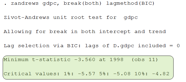
- none of the variable should be I(2) in structural break (Zivot Andrews test)
Step 1 Check Optimal Lag order
First we need to check the lag order to see what lag we use to the ADF test for each variable which is being used in the model. This is done using VARSOC Table (Vector Auto Regressive Specification Order Criterion) which is available in STATA that can be quickly applied, in EVIEWS you have to do it after VAR model and check the Lag length criterion, you can learn that from this blog post by Dave Giles.
To learn how to import and handle data in STATA visit

This test will provide 6 methods (LL, LR(p), FPE, AIC, HQIC, SBIC) and there will be a star on them where that criteria had optimal lag, so we need to select the majority so here the lag order is 1 for this variable. Similarly you have to find optimal lags for all variables. The code of this in STATA is “varsoc variable-name”
Check the stationarity of each variable
Now we need to confirm if none of the variable is I(2) for this we need to do the ADF Test (Augmented Dickey Fuller) and see the Z(t) statistic on the top if the first test statistic is smaller than all others in magnitude if they have same sign then it means that variable is I(1) when we are checking at level. similarly you have to prove it I(0) at first difference.

See in the table of first difference now the test statistic is larger than at least one of the critical value so it is I(0) at first difference.

Next is to see if the variable is sensitive to structural break means to say if we check unit root (Zivot Andrews Test) in the test that allows structural break then if the variable shows to be I(2) then there is a problem that needed to be addressed like we might have to add a structural break variable in the model or we have to remove the break from the variable. It is checked and interpreted same as the ADF Test.
Now once you proved that all variables are not I(2) you can proceed to ARDL model. This document will help you to do ARDL estimation in Microfit. Firstly we have to import data in Microfit. It can be done by first coping all the data with variable names without spaces and the years. Then open Microfit and go in file and select copy data from the clipboard. it will show you the data press OK there.
It will ask if you have years on the left most column if you have copied the years to the select it, then if you have selected the names of the variables while coping then select here too and as there was no description of the variables in the copied file then select no description and press OK.
you can get Microfit 5 from here
you will see your variable names in the center in red like in the picture below

now you need to add the intercept and the trend term which might be used in the estimation for intercept press the constant term below at right it will ask what name you want to give to it, I usually change it to “c” so that it is small as possible. For trend press the time trend button and it will ask to name it , i usually keep it as “t” only so that it is small too. After this your data is ready for estimation of ARDL; go in uni-variate on the top and press ARDL approach to cointegration; it will show you the estimation page like image below

here you have to mention the names of your variables (same spelling as you had in the excel file without spaced it is good to keep them small as possible so that it is easy to remember and retype) in appropriate order dependent first and all others after it. And at the end enter “&” and enter c for constant and t for trend (if needed) this “&” sign will differentiate between variables and constants (exogenous) in Microfit. When you entered variable names press run on the right top with here the lag order of ARDL is 1 so try to make the model at 1 lag order first if not then we will see lag order 2.
When u press run it will take some times at it is a DEMO version to press OK for few times if there is any error then it will show you one menu (let’s call it menu 1 for selecting lag order criterion) like this below

here you have to mention the method you want to use let it be Schwarz Bayesian criterion as standard and press ok (you can specify you own ARDL order at 6 if any one of the above criterion are not giving appropriate diagnostics, you can make you own from you unit root results as you know all I(0) are not related to past so their lag order must be zero and others can be one. and second method is to see in the ARDL results whose level is significant so we do not need its lag so actually it is hit and trial method if you have studied time series you might have intuition behind how to find the appropriate lag if any of the criterion are not able to provide suitable results)
After a little time it will show you another menu (let it call menu to for ARDL model selection) like this

here you first have to see the ADRL regression for fitness so press OK by selecting option 1. it will show you results like this

In this table you have to note the highlighted things first and for most you have to see if the F-statistic (of 5.85) is higher than the upper bound at 95% (of 4.82) or 90% (of 3.87) any one will work. If it comes higher, then you can say that there is cointegration among the set of (I(0) & I(1)) variables so we can assume that there can be at least long run or short run relation among these variables. If this F statistic is not higher than any of the upper bound critical values for first try to modify the lag order so that F statistic might go above the critical value of upper bound if it is not possible see the guide in following passage.
If the F statistic is higher than the lower bound but lower than the upper bound then you must check all of your I(1) variables if there is any useless (to remove) or you have missed any one (to add) . if F statistic is lower than the lower bound then all of your variables I(0) and I(1) are not appropriate means to they are not cointegrated try to change the model add more variables modify their specification if possible other wise you can report that these variables do not relate with each other their relationship is spurious.
So if you found the F statistic larger than the upper bound like in the image above then you have to see the diagnostics there are four provided at the end of the table (which are auto-correlation, normality, specification and hetroskedasticity test) first is serial correlation which is insignificant as per F version but significant at 5% in LM version so we can assume that there is no auto-correlation at 1% or according to F version. Similarly the functional form is insignificant (no issue); normality is insignificant (no issue) and hetroskedasticity is insignificant (no issue) too hence there is no apparent issue which with this model. So we can proceed to next step.
If you find any of the issue try to change the lag order increase sample or variable specification in order to correct them. if your sample is higher than the 30 then you can ignore the normality issue if it exists as per central limit theorem. There is another information on the top of the table which is the lag order of the estimation which is to be reported in the regression analysis. Press close to proceed it will show you a new menu (call it menu 3 of post regression) like this

Here select the second option of move to hypothesis testing menu as we need to see if there is any recursive residuals because of structural break as ARDL is sensitive to it. When you press OK you will see another menu (let it be menu 4 of hypothesis testing) like this

Here you need to use the CUSUM and CUSUMSQ charts which is at option 4 select it and press OK it will show you two charts one by one by pressing CLOSE button copy them in your estimation document, they look like following . The thing to note here is that the blue line must not cross red and the green one for any of both charts. If it does not cross then it means that there is not issue of recursive residuals in terms of mean (in first CUSUM chart) and in terms of variance (in second CUSUMSQ chart) so you can proceed . If you find issue here then you must have added some variable which is sensitive to structural break, it might be solved if you add the trend otherwise you have to find the structural break of the dependent variable and make dummy from it and introduce it as independent variable in order to balance the residuals.


When you close both charts it will show you the 4th menu again you have to go back so select 0 option, now it will show you the 3rd menu you have to go back again so press 0 option and OK, now here you want to see the long run results are the model as it has passed the diagnostics (F statistic, auto-correlation, hetroskedasticity, specification, normality, CUSUM and CUSUMSQ).
It will show you results like following. you have to note the highlighted things as they are the long run estimates so use the coefficient and its t value and probability to interpret the model in long run. Here most of them are insignificant it does not means that model is bad they are cointegrating as we have seen from the f statistic in the first table so they might be effecting each other in short run if they are not in long run.

These results can be written as where the green one is significant
LGDP = – 0.70 + 0.64 LFDI – 0.003 TRA + 0.22 INF – 0.04 CRED + 0.002 MC
t values -0.23 2.83 -0.71 1.68 -1.32 0.86
prob 0.81 0.01 0.49 0.11 0.20 0.41
Press close you are on the 3rd menu again go back to 2nd menu by pressing 0 option and OK. Now you want to see the error correction model to see the short run results, it will show you results like following

Here you have to note the following see the estimates on the top of the table they are short run components. here ecm(-1) is most important it should at least be negative and significant also if it is between 0 and -1 then it will be ideal (this conditions will ensure that there is convergence in the model which indirectly means that there is a significant long run relation)
So here it is significant at 10% level and between 0 and -1 , it is -0.11 the more it is near to -1 stronger the equilibrium is but its significance is must. So we have proven equilibrium though it is weak or slow. rest of the variables are showing the short run component, the significant variables will show that they have significant effect on the dependent variable in short run. if some variable have both short run and long run components significant they we can say that the particular variable has strong causal effect on the dependent other wise of it is short run only then it is weak causal effect. It is reported as
ΔLGDP = 0.07 ΔLFDI + 0.0002 ΔTRA + 0.03 ΔINF – 0.01 ΔCRED + 0.0003 ΔMC – 0.12 ECM(-1)
t values 2.66 0.25 2.82 -4.24 0.81 -1.78
prob 0.02 0.80 0.01 0.00 0.43 0.09
Other things to note is the r square and the F test. R square is for interpretation like OLS and F test to see overall fitness of the model if the model is too weak then it will become insignificant, here another thing is the residual sum of squares which can be use to compare it with some other ARDL model with same dependent variable if we want to see performance of two models then we compare this. Here you cannot interpret the Durban Watson as there are lags in the model so no need to worry about it as the serial auto test has cleared the presence of auto in the first table. In this model of short run FDI, Inf, Cred are significant. So this is your model of ARDL there are one more step that is usually done in order to see if the ARDL model is consistent or not. See the above example it is GDP = f(FDI, TRA, INF, CRED, MC) so the F test in the first table led to clarify that this model is true and valid but it does not tell any thing about the reverse models like.
FDI = f(GDP, TRA, INF, CRED, MC)
TRA = f(FDI, GDP, INF, CRED, MC)
INF = f(FDI, TRA, GDP, CRED, MC)
CRED = f(FDI, TRA, INF, GDP, MC)
MC = f(FDI, TRA, INF, CRED, GDP)
So if any one of these models are also true and valid then this ARDL results we have found will become inconsistent, means to say that this approach is single equation model but there are more than two equations that needed to be estimated which require simultaneous equation model. That is why it was advised at the start that if all variables are I(1) then Johanson Approach ECM can be a use-full method. So we check the consistency of the model by running these 5 mentioned models in Microfit and see their F – Test values in the first table just like we did in the above example and hope and for all these 5 models the F test values are lower than the lower bound values.
If you want to see its details see the following links
Detail ARDL model by Dave Giles
Learn it from video
This attempt to explain ARDL is preliminary subject to improve based on the comments and suggestions below. If you think that there is a room for improvement let me know because we can change the description above any time unlike a book which cannot me modified after being published. In order to polish your skill of ARDL it is good to see articles on it after reading the blog and see how people have presented it and explained i
No comments:
Post a Comment