The Dickey-Fuller (DF) Unit Root Test in an AR(1) Model

ARDL Models - Part II - Bounds Tests

ARDL Models - Part II - Bounds Tests

http://davegiles.blogspot.in/2013/06/ardl-models-part-ii-bounds-tests.html

[Note: For an important update of this post, relating to EViews 9, see my 2015 post, here.]

Well, I finally got it done! Some of these posts take more time to prepare than you might think.

The first part of this discussion was covered in a (sort of!) recent post, in which I gave a brief description of Autoregressive Distributed Lag (ARDL) models, together with some historical perspective. Now it's time for us to get down to business and see how these models have come to play a very important role recently in the modelling of non-stationary time-series data.

In particular, we'll see how they're used to implement the so-called "Bounds Tests", to see if long-run relationships are present when we have a group of time-series, some of which may be stationary, while others are not. A detailed worked example, using EViews, is included.

First, recall that the basic form of an ARDL regression model is:

           y_t = β₀ + β₁y_t-1 + .......+ β_ky_t-p + α₀x_t + α₁x_t-1 + α₂x_t-2 + ......... + α_qx_t-q + ε_t ,      (1)

where ε_t is a random "disturbance" term, which we'll assume is "well-behaved" in the usual sense. In particular, it will be serially independent.

We're going to modify this model somewhat for our purposes here. Specifically, we'll work with a mixture of differences and levels of the data. The reasons for this will become apparent as we go along.

Let's suppose that we have a set of time-series variables, and we want to model the relationship between them, taking into account any unit roots and/or cointegration associated with the data. First, note that there are three straightforward situations that we're going to put to one side, because they can be dealt with in standard ways:

1. We know that all of the series are I(0), and hence stationary. In this case, we can simply model the data in their levels, using OLS estimation, for example.
2. We know that all of the series are integrated of the same order (e.g., I(1)), but they are not cointegrated. In this case, we can just (appropriately) difference each series, and estimate a standard regression model using OLS.
3. We know that all of the series are integrated of the same order, and they are cointegrated. In this case, we can estimate two types of models: (i) An OLS regression model using the levels of the data. This will provide the long-run equilibrating relationship between the variables. (ii) An error-correction model (ECM), estimated by OLS. This model will represent the short-run dynamics of the relationship between the variables.

1. Now, let's return to the more complicated situation mentioned above. Some of the variables in question may be stationary, some may be I(1) or even fractionally integrated, and there is also the possibility of cointegration among some of the I(1) variables. In other words, things just aren't as "clear cut" as in the three situations noted above.

What do we do in such cases if we want to model the data appropriately and extract both long-run and short-run relationships? This is where the ARDL model enters the picture.

The ARDL / Bounds Testing methodology of Pesaran and Shin (1999) and Pesaran et al. (2001) has a number of features that many researchers feel give it some advantages over conventional cointegration testing. For instance:

• It can be used with a mixture of I(0) and I(1) data.
• It involves just a single-equation set-up, making it simple to implement and interpret.
• Different variables can be assigned different lag-lengths as they enter the model.

We need a road map to help us. Here are the basic steps that we're going to follow (with details to be added below):

1. Make sure than none of the variables are I(2), as such data will invalidate the methodology.
2. Formulate an "unrestricted" error-correction model (ECM). This will be a particular type of ARDL model.
3. Determine the appropriate lag structure for the model in step 2.
4. Make sure that the errors of this model are serially independent.
5. Make sure that the model is "dynamically stable".
6. Perform a "Bounds Test" to see if there is evidence of a long-run relationship between the variables.
7. If the outcome at step 6 is positive, estimate a long-run "levels model", as well as a separate "restricted" ECM.
8. Use the results of the models estimated in step 7 to measure short-run dynamic effects, and the long-run equilibrating relationship between the variables.

We can see from the form of the generic ARDL model given in equation (1) above, that such models are characterised by having lags of the dependent variable, as well as lags (and perhaps the current value) of other variables, as the regressors. Let's suppose that there are three variables that we're interested in modelling: a dependent variable, y, and two other explanatory variables, x₁ and x₂. More generally, there will be (k + 1) variables - a dependent variable, and k other variables.

Before we start, let's recall what a conventional ECM for cointegrated data looks like. It would be of the form:

          Δy_t = β₀ + Σ β_iΔy_t-i + Σγ_jΔx_1t-j + Σδ_kΔx_2t-k + φz_t-1 + e_t    ;        (2)

Here, z, the "error-correction term", is the OLS residuals series from the long-run "cointegrating regression",

           y_t = α₀ + α₁x_1t + α₂x_2t + v_t       ;       (3)

The ranges of summation in (2) are from 1 to p, 0 to q₁, and 0 to q₂ respectively.

Now, back to our own analysis-

Step 1:
We can use the ADF and KPSS tests to check that none of the series we're working with are I(2).

Step 2:

Formulate the following model:

    Δy_t = β₀ + Σ β_iΔy_t-i + Σγ_jΔx_1t-j + Σδ_kΔx_2t-k + θ₀y_t-1 + θ₁x_1t-1 + θ₂ x_2t-1 + e_t   ;    (4)

Notice that this is almost like a traditional ECM. The difference is that we've now replaced the error-correction term, z_t-1 with the terms y_t-1, x_1t-1, and x_2t-1. From (3), we can see that the lagged residuals series would be z_t-1 = (y_t-1 - a₀ - a₁x_1t-1- a₂x_2t-1), where the a's are the OLS estimates of the α's. So, what we're doing in equation (4) is including the same lagged levels as we do in a regular ECM, but we're not restricting their coefficients.

This is why we might call equation (4) an "unrestricted ECM", or an "unconstrained ECM". Pesaran et al. (2001) call this a "conditional ECM".

Step 3:

The ranges of summation in the various terms in (4) are from 1 to p, 0 to q₁, and 0 to q₂ respectively.We need to select the appropriate values for the maximum lags, p, q₁, and q₂. Also, note that the "zero lags" on Δx₁ and Δx₂ may not necessarily be needed. Usually, these maximum lags are determined by using one or more of the "information criteria" - AIC, SC (BIC), HQ, etc. These criteria are based on a high log-likelihood value, with a "penalty" for including more lags to achieve this. The form of the penalty varies from one criterion to another. Each criterion starts with -2log(L), and then penalizes, so the smaller the value of an information criterion the better the result.

I generally use the Schwarz (Bayes) criterion (SC), as it's a consistent model-selector. Some care has to be taken not to "over-select" the maximum lags, and I usually also pay some attention to the (apparent) significance of the coefficients in the model.

Step 4:
A key assumption in the ARDL / Bounds Testing methodology of Pesaran et al. (2001) is that the errors of equation (4) must be serially independent. As those authors note (p.308), this requirement may also be influential in our final choice of the maximum lags for the variables in the model.

Once an apparently suitable version of (4) has been estimated, we should use the LM test to test the null hypothesis that the errors are serially independent, against the alternative hypothesis that the errors are (either) AR(m) or MA(m), for m = 1, 2, 3,...., etc.

Step 5:
We have a model with an autoregressive structure, so we have to be sure that the model is "dynamically stable". For full details of what this means, see my recent post, When is an Autoregressive Model Dynamically Stable? What we need to do is to check that all of the inverse roots of the characteristic equation associated with our model lie strictly inside the unit circle. That recent post of mine showed how to trick EViews into giving us the information we want in order to check that this condition is satisfied. I won't repeat that here.

Step 6:
Now we're ready to perform the "Bounds Testing"!

Here's equation (4), again:

      Δy_t = β₀ + Σ β_iΔy_t-i + Σγ_jΔx_1t-j + Σδ_kΔx_2t-k + θ₀y_t-1 + θ₁x_1t-1 + θ₂ x_2t-1 + e_t   ;    (4)

All that we're going to do is preform an "F-test" of the hypothesis, H₀:  θ₀ = θ₁ = θ₂ = 0 ; against the alternative that H₀  is not true. Simple enough - but why are we doing this?

As in conventional cointegration testing, we're testing for the absence of a long-run equilibrium relationship between the variables. This absence coincides with zero coefficients for y_t-1, x_1t-1 and x_2t-1 in equation (4). A rejection of H₀ implies that we have a long-run relationship.

There is a practical difficulty that has to be addressed when we conduct the F-test. The distribution of the test statistic is totally non-standard (and also depends on a "nuisance parameter", the cointegrating rank of the system) even in the asymptotic case where we have an infinitely large sample size.  (This is somewhat akin to the situation with the Wald test when we test for Granger non-causality in the presence of non-stationary data. In that case, the problem is resolved by using the Toda-Yamamoto (1995) procedure, to ensure that the Wald test statistic is asymptotically chi-square, as discussed here.)

Exact critical values for the F-test aren't available for an arbitrary mix of I(0) and I(1) variables. However, Pesaran et al. (2001) supply bounds on the critical values for the asymptotic distribution of the F-statistic. For various situations (e.g., different numbers of variables, (k + 1)), they give lower and upper bounds on the critical values. In each case, the lower bound is based on the assumption that all of the variables are I(0), and the upper bound is based on the assumption that all of the variables are I(1). In fact, the truth may be somewhere in between these two polar extremes.

If the computed F-statistic falls below the lower bound we would conclude that the variables are I(0), so no cointegration is possible, by definition. If the F-statistic exceeds the upper bound, we conclude that we have cointegration. Finally, if the F-statistic falls between the bounds, the test is inconclusive.

Does this remind you of the old Durbin-Watson test for serial independence? It should!

As a cross-check, we should also perform a "Bounds t-test" of H₀ : θ₀ = 0, against H₁ :  θ₀ < 0. If the t-statistic for y_t-1 in equation (4) is greater than the "I(1) bound" tabulated by Pesaran et al. (2001; pp.303-304), this would support the conclusion that there is a long-run relationship between the variables. If the t-statistic is less than the "I(0) bound", we'd conclude that the data are all stationary.

Step 7:
Assuming that the bounds test leads to the conclusion of cointegration, we can meaningfully estimate the long-run equilibrium relationship between the variables:

            y_t = α₀ + α₁x_1t + α₂x_2t + v_t       ;      (5)

as well as the usual ECM:

          Δy_t = β₀ + Σ β_iΔy_t-i + Σγ_jΔx_1t-j + Σδ_kΔx_2t-k + φz_t-1 + e_t    ;    (6)

where z_t-1 = (y_t-1 -a₀ - a₁x_1t-1 - a₂x_2t-1), and the a's are the OLS estimates of the α's in (5).

Step 8:
We can "extract" long-run effects from the unrestricted ECM. Looking back at equation (4), and noting that at a long-run equilibrium,  Δy_t = 0, Δx_1t = Δx_2t = 0, we see that the long-run coefficients for x₁ and x₂ are -(θ₁/ θ₀) and -(θ₂/ θ₀) respectively.

An Example:
Now we're ready to look at a very simple empirical example. I'm going to use the data for U.S. and European natural gas prices that I made available as a second example in my post, Testing for Granger Causality. I didn't go through the details of testing for Granger causality with that set of data, but I mentioned near the end of the post, and the EViews file (which included a "read_me" object with comments about the results) is there on the code page for this blog (dated 29 April, 2011).

If you look back at that earlier file, you'll find that I used the Toda-Yamamoto (1995) testing procedure to determine that there is Granger causality running from the U.S. series to the European series, but not vice versa.

A new EViews file that uses the same data for our ARDL modelling is available on the code page, under the date for the current post. The data for the two time-series we'll be using are also available on the data page for this blog. The data are monthly, from 1995(01) to 2011(03). In terms of the notation that was introduced earlier, we have (k + 1) = 2 variables, so k = 1 when it comes to the bounds testing.

Here's a plot of the data we'll be using (remember that you can enlarge most of these inserts by clicking on them):

To complete Step 1, we need to check that neither of our time-series are I(2). Applying the ADF test to the levels of EUR and US, the p-values are 0.53 and 0.10 respectively. Applying the test to the first-differences of the series, the p-values are both 0.00. (The lag-lengths for the ADF regressions were chosen using the Schwarz criterion, SC.) Clearly, neither series is I(2).

Applying the KPSS test we  reject the null of stationarity, even at the 1% significance level, for both EUR and US, but cannot reject the null of I(1) against I(2). The p-value of 10% for the ADF test of I(1) vs. I(0) for the EUR series may leave us wondering if that series is stationary, or not. You'll know that apparent "conflicts" between the outcomes of tests such as these are very common in practice.

This is a great illustration of how the ARDL / Bounds Testing methodology can help us. In order for standard cointegration testing (such as that of Engle and Granger, or Johansen) to make any sense, we must be really sure that all of the series are integrated of the same order. In this instance, you might not be feeling totally sure that this is the case.

Step 2 is straightforward. Given that the Granger causality testing associated with my earlier post suggested that there is causality from US to EUR (but not vice versa), ΔEUR is going to be the dependent variable in my unrestricted ECM:

          ΔEUR_t = β₀ + Σ β_iΔEUR_t-i + Σγ_jΔUS_t-j + θ₀EUR_t-1 + θ₁US_t-1 + e_t   ;     (5)

That's Step 2 out of the way!

To implement the information criteria for selecting the lag-lengths in an time-efficient way, I "tricked" EViews into providing lots of them at once by doing the following. I estimated a 1-equation VAR model for ΔEUR_t and I supplied the intercept, EUR_t-1, US_t-1, and a fixed number of lags of ΔUS_t as exogenous regressors. For example, when the fixed number of lags on ΔUS_t was zero, here's how I specified the VAR:

After estimating this model, I then chose VIEW, LAG STRUCTURE, LAG LENGTH CRITERIA:

I then repeated this by adding  ΔUS_t-1 to the list of exogenous variables, and got the following results:

I proceeded in this manner with additional lags of ΔUS_t in the "exogenous" list. I also considered cases such as:

which resulted in the following information criteria values:

Looking at the SC values in these three tables of results, we see that a maximum lag of 4 is suggested for ΔEUR_t. (The AIC values suggest that 8 lags of ΔEUR_t may be appropriate, but some experimentation with this was not fruitful.)

There is virtually no difference between the SC values for the case where the model includes just US_t as a regressor (0.8714), and the case where just ΔUS_t-1 is included (0.8718). To get some dynamics into the model, I'm going to go with the latter case.

With Step 3 completed, and with this lag specification in mind, let's now look at the estimated unrestricted ECM:

Step 4 involves checking that the errors of this model are serially independent. Selecting VIEW, RESIDUAL DIAGNOSTICS, SERIAL CORRELATION LM TEST, I get the following results:

m           LM         p-value

1           0.079        0.779

2           2.878        0.237

3           5.380        0.146

4         11.753        0.019

O.K., we have a problem with serial correlation! To deal with it, I experimented with one or two additional lags of the dependent variable as regressors, and ended up with the following specification for the unrestricted ECM:

The serial independence results now look much more satisfactory:

m           LM         p-value

1           0.013        0.911

2           3.337        0.189

3           5.183        0.159

4           7.989        0.092

5           8.473        0.132

6         11.023        0.088

7         12.270        0.092

8         12.334        0.137

Next, Step 5 involves checking the dynamic stability of this ARDL model. Here are the inverse roots of the associated characteristic equation:

All seems to be well - these roots are all inside the unit circle.

Before proceeding to the Bounds Testing, let's take a look at the "fit" of our unrestricted ECM. The "Actual / Fitted / Residuals" plot looks like this:

When we "unscramble" these results, and look at the fit of the model in terms of explaining the level of EUR itself, rather than ΔEUR, things look pretty good: 

We're now ready for Step 6 - the Bounds Test itself. We want to test if the coefficients of both EUR(-1) and US(-1) are zero in our estimated model (repeated below):

 

The associated F-test is obtained as follows:

With the result:

The value of our F-statistic is 5.827, and we have (k + 1) = 2 variables (EUR and US) in our model. So, when we go to the Bounds Test tables of critical values, we have k = 1.

Table CI (iii) on p.300 of Pesaran et al. (2001) is the relevant table for us to use here. We haven't constrained the intercept of our model, and there is no linear trend term included in the ECM.  The lower and upper bounds for the F-test statistic at the 10%, 5%, and 1% significance levels are [4.04 , 4.78], [4.94 , 5.73], and [6.84 , 7.84] respectively. 

As the value of our F-statistic exceeds the upper bound at the 5% significance level, we can conclude that there is evidence of a long-run relationship between the two time-series (at this level of significance or greater). 

In addition, the t-statistic on EUR(-1) is -2.926. When we look at Table CII (iii) on p.303 of Pesaran et al. (2001), we find that the I(0) and I(1) bounds for the t-statistic at the 10%, 5%, and 1% significance levels are [-2.57 , -2.91], [-2.86 , -3.22], and [-3.43 , -3.82] respectively. At least at the 10% significance level, this result reinforces our conclusion that there is a long-run relationship between EUR and US.

So, here we are at Step 7 and Step 8.

Recalling our preferred unrestricted ECM:

we see that the long-run multiplier between US and EUR is -(0.047134 / (-0.030804)) = 1.53. In the long run, an increase of 1 unit in US will lead to an increase of 1.53 units in EUR.

If we estimate the levels model,

                   EUR_t = α₀ + α₁US_t + v_t       ,

by OLS, and construct the residuals series, {z_t}, we can fit a regular (restricted) ECM:

Notice that the coefficient of the error-correction term, z_t-1, is negative and very significant. This is what we'd expect if there is cointegration between EUR and US. The magnitude of this coefficient implies that nearly 3% of any disequilibrium between EUR and US is corrected within one period (one month).

This final ECM is dynamically stable:

As none of the roots lie on the X (real) axis, it's clear that we have three complex conjugate pairs of roots. Accordingly, the short-run dynamics associated with the model are quite complicated. This can be seen if we consider the impulse response function associated with a "shock" of one (sample) standard deviation:

Finally, the within-sample fit (in terms of the levels of EUR) is exceptionally good:

In fact, the simple correlations between EUR and the "fitted" EUR series from the unrestricted and regular ECM's are each 0.994, and the correlation between the two fitted series is 0.9999.

So, there we have it - bounds testing with an ARDL model.

[Note: For an important update of this post, relating to EViews 9, see my 2015 post, here.]

References

Pesaran, M. H. and Y. Shin, 1999. An autoregressive distributed lag modelling approach to cointegration analysis. Chapter 11 in S. Strom (ed.), Econometrics and Economic Theory in the 20th Century: The Ragnar Frisch Centennial Symposium. Cambridge University Press, Cambridge. (Discussion Paper version.)

Pesaran, M. H., Shin, Y. and Smith, R. J., 2001. Bounds testing approaches to the analysis of level relationships. Journal of Applied Econometrics, 16, 289–326.

Pesaran, M. H. and R. P. Smith, 1998. Structural analysis of cointegrating VARs. Journal of Economic Surveys, 12, 471-505.

Toda, H. Y and T. Yamamoto (1995). Statistical inferences in vector autoregressions with possibly integrated processes. Journal of Econometrics, 66, 225-250.

© 2013, David E. Giles

A manual for ARDL approach to cointegration

A manual for ARDL approach to cointegration

ARDL model was introduced by Pesaran et al. (2001) in order to incorporate I(0) and I(1) variables in same estimation so if your variables are stationary I(0) then OLS is appropriate and if all are non stationary I(1) then it is advisable to do VECM (Johanson Approach) as it is much simple model.

We cannot estimate conventional OLS on the variables if any one of them or all of them are (1) because these variable will not behave like constants which is required in OLS and as most of then are changing in time so OLS will mistakenly show high t values and significant results but in reality it would be inflated because of common time component, in econometric it is called spurious results where R square of the model becomes higher than the Durban Watson Statistic. So we move to a new set of models which can work on I(1) variables.

How to Estimate ARDL model

In order to run ARDL some preconditions needed to be checked

• Dependent must be non stationary in order for the model to behave better.
• None of the variable should be I(2) in normal conditions (ADF test)
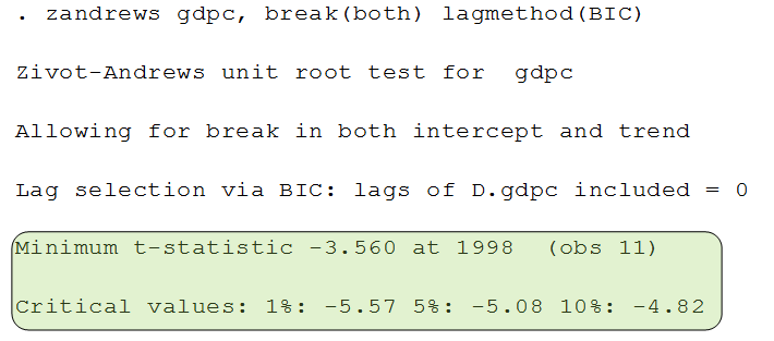
• none of the variable should be I(2) in structural break (Zivot Andrews test)

Step 1 Check Optimal Lag order

First we need to check the lag order to see what lag we use to the ADF test for each variable which is being used in the model.  This is done using VARSOC Table (Vector Auto Regressive Specification Order Criterion) which is available in STATA that can be quickly applied, in EVIEWS you have to do it after VAR model and check the Lag length criterion, you can learn that from this blog post by Dave Giles.

To learn how to import and handle data in STATA visit

http://econistics.wix.com/home#!Chapter-1-Importing-data-in-STATA/cgor/90096572-0B0D-4832-9AFD-51C18A0017F0

This test will provide 6 methods (LL, LR(p), FPE, AIC, HQIC, SBIC) and there will be a star on them where that criteria had optimal lag, so we need to select the majority so here the lag order is 1 for this variable. Similarly you have to find optimal lags for all variables. The code of this in STATA is “varsoc variable-name”

Check the stationarity of each variable

Now we need to confirm if none of the variable is I(2) for this we need to do the ADF Test (Augmented Dickey Fuller)  and see the Z(t) statistic on the top if the first test statistic is smaller than all others in magnitude if they have same sign then it means that variable is I(1) when we are checking at level. similarly you have to prove it I(0) at first difference.

See in the table of first difference now the test statistic is larger than at least one of the critical value so it is I(0) at first difference.

Next is to see if the variable is sensitive to structural break means to say if we check unit root (Zivot Andrews Test) in the test that allows structural break then if the variable shows to be I(2) then there is a problem that needed to be addressed like we might have to add a structural break variable in the model or we have to remove the break from the variable. It is checked and interpreted same as the ADF Test.

Now once you proved that all variables are not I(2) you can proceed to ARDL model. This document will help you to do ARDL estimation in Microfit. Firstly we have to import data in Microfit. It can be done by  first coping all the data with variable names without spaces and the years. Then open Microfit and go in file and select copy data from the clipboard. it will show you the data press OK there.

It will ask if you have years on the left most column if you have copied the years to the select it, then if you have selected the names of the variables while coping then select here too and as there was no description of the variables in the copied file then select no description and press OK.

you can get Microfit 5 from here

https://www.dropbox.com/s/r0viysvisecldho/Setup_Demo%20microfit%205.rar?dl=0

you will see your variable names in the center in red like in the picture below

now you need to add the intercept and the trend term which might be used in the estimation for intercept press the constant term below at right it will ask what name you want to give to it, I usually change it to “c” so that it is small as possible. For trend press the time trend button and it will ask to name it , i usually keep it as “t” only so that it is small too. After this your data is ready for estimation of ARDL; go in uni-variate on the top and press ARDL approach to cointegration; it will show you the estimation page like image below

here you have to mention the names of your variables (same spelling as you had in the excel file without spaced it is good to keep them small as possible so that it is easy to remember and retype) in appropriate order dependent first and all others after it.  And at the end enter “&” and enter c for constant and t for trend (if needed) this “&” sign will differentiate between variables and constants (exogenous) in Microfit. When you entered variable names press run on the right top with here the lag order of ARDL is 1 so try to make the model at 1 lag order first if not then we will see lag order 2.

When u press run it will take some times at it is a DEMO version to press OK for few times if there is any error then it will show you one menu (let’s call it menu 1 for selecting lag order criterion) like this below

here you have to mention the method you want to use let it be Schwarz Bayesian criterion as standard and press ok (you can specify you own ARDL order at 6 if any one of the above criterion are not giving appropriate diagnostics, you can make you own from you unit root results as you know all I(0) are not related to past so their lag order must be zero and others can be one. and second method is to see in the ARDL results whose level is significant so we do not need its lag so actually it is hit and trial method if you have studied time series you might have intuition behind how to find the appropriate lag if any of the criterion are not able to provide suitable results)

After a little time it will show you another menu  (let it call menu to for ARDL model selection) like this

here you first have to see the ADRL regression for fitness so press OK by selecting option 1. it will  show you results like this

In this table you have to note the highlighted things first and for most you have to see if the F-statistic (of 5.85) is higher than the upper bound at 95% (of 4.82) or 90%  (of 3.87) any one will work. If it comes higher, then you can say that there is cointegration among the set of (I(0) & I(1)) variables so we can assume that there can be at least long run or short run relation among these variables. If this F statistic is not higher than any of the upper bound critical values for first try to modify the lag order so that F statistic might go above the critical value of upper bound if it is not possible see the guide in following passage.

If the F statistic is higher than the lower bound but lower than the upper bound then you must check all of your I(1) variables if there is any useless (to remove) or you have missed any one (to add) . if F statistic is lower than the lower bound then all of your variables  I(0) and I(1) are not appropriate means to they are not cointegrated try to change the model add more variables modify their specification if possible other wise you can report that these variables do not relate with each other their relationship is spurious.

So if you found the F statistic larger than the upper bound like in the image above then you have to see the diagnostics there are four provided at the end of the table (which are auto-correlation, normality, specification and hetroskedasticity test) first is serial correlation which is insignificant as per F version but significant at 5% in LM version so we can assume that there is no auto-correlation at 1% or according to F version. Similarly the functional form is insignificant (no issue); normality is insignificant (no issue) and hetroskedasticity is insignificant (no issue) too hence there is no apparent issue which with this model. So we can proceed to next step.

If you find any of the issue try to change the lag order increase sample or variable specification in order to correct them.  if your sample is higher than the 30 then you can ignore the normality issue if it exists as per central limit theorem. There is another information on the top of the table which is the lag order of the estimation which is to be reported in the regression analysis. Press close to proceed it will show you a new  menu (call it menu 3 of post regression) like this

Here select the second option of move to hypothesis testing menu as we need to see if there is any recursive residuals because of structural break as ARDL is sensitive to it. When you press OK you will see another menu (let it be menu 4 of hypothesis testing) like this

Here you need to use the CUSUM and CUSUMSQ charts which is at option 4 select it and press OK  it will show you two charts one by one by pressing CLOSE button copy them in your estimation document, they look like following . The thing to note here is that the blue line must not cross red and the green one for any of both charts. If it does not cross then it means that there is not issue of recursive residuals in terms of mean (in first CUSUM chart) and in terms of variance (in second CUSUMSQ chart) so you can proceed . If you find issue here then you must have added some variable which is sensitive to structural break, it might be solved if you add the trend otherwise you have to find the structural break of the dependent variable and make dummy from it and introduce it as independent variable in order to balance the residuals.

When you close both charts it will show you the 4th menu again you have to go back so select 0 option, now it will show you the 3rd menu you have to go back again so press 0 option and OK, now here you want to see the long run results are the model as it has passed the diagnostics (F statistic, auto-correlation, hetroskedasticity, specification, normality, CUSUM and CUSUMSQ).

It will show you results like following. you have to note the highlighted things as they are the long run estimates so use the coefficient and its t value and probability to interpret the model in long run. Here most of them are insignificant it does not means that model is bad they are cointegrating as we have seen from the f statistic in the first table so they might be effecting each other in short run if they are not in long run.

These results can be written as where the green one is significant

LGDP = – 0.70  + 0.64 LFDI – 0.003 TRA + 0.22 INF – 0.04 CRED + 0.002 MC

t values   -0.23      2.83               -0.71                  1.68             -1.32              0.86

prob         0.81       0.01                0.49                  0.11              0.20               0.41

Press close you are on the 3rd menu again go back to 2nd menu by pressing 0 option and OK. Now you want to see the error correction model to see the short run results, it will show you results like following

Here you have to note the following see the estimates on the top of the table they are short run components. here ecm(-1) is most important it should at least be negative and significant also if it is between 0 and -1 then it will be ideal (this conditions will ensure that there is convergence in the model which indirectly means that there is a significant long run relation)

So here it is significant at 10% level and between 0 and -1 , it is -0.11 the more it is near to -1 stronger the equilibrium is but its significance is must. So we have proven equilibrium though it is weak or slow. rest of the variables are showing the short run component, the significant variables will show that they have significant effect on the dependent variable in short run.  if some variable have both short run and long run components significant they we can say that the particular variable has strong causal effect on the dependent other wise of it is short run only then it is weak causal effect. It is reported as

ΔLGDP =  0.07 ΔLFDI + 0.0002 ΔTRA + 0.03 ΔINF – 0.01 ΔCRED + 0.0003 ΔMC – 0.12 ECM(-1)

t values     2.66                   0.25                      2.82                  -4.24               0.81                    -1.78

prob           0.02                  0.80                      0.01                  0.00                 0.43                    0.09

Other things to note is the r square and the F test. R square is for interpretation  like OLS and F test to see overall fitness of the model if the model is too weak then it will become insignificant, here another thing is the residual sum of squares which can be use to compare it with some other ARDL model with same dependent variable if we want to see performance of two models then we compare this. Here you cannot interpret the Durban Watson as there are lags in the model so no need to worry about it as the serial auto test has cleared the presence of auto in the first table. In this model of short run FDI, Inf, Cred are significant. So this is your model of ARDL there are one more step that is usually done in order to see if the ARDL model is consistent or not. See the above example it is GDP = f(FDI, TRA, INF, CRED, MC) so the F test in the first table led to clarify that this model is true and valid but it does not tell any thing about the reverse models like.

FDI = f(GDP, TRA, INF, CRED, MC)

TRA = f(FDI, GDP, INF, CRED, MC)

INF = f(FDI, TRA, GDP, CRED, MC)

CRED = f(FDI, TRA, INF, GDP, MC)

MC = f(FDI, TRA, INF, CRED, GDP)

So if any one of these models are also true and valid then this ARDL results we have found will become inconsistent, means to say that this approach is single equation model but there are more than two equations that needed to be estimated which require simultaneous equation model. That is why it was advised at the start that if all variables are  I(1) then Johanson Approach ECM can be a use-full method. So we check the consistency of the model by running these 5 mentioned models in Microfit and see their F – Test values in the first table just like we did in the above example and hope and for all these 5 models the F test values are lower than the lower bound values.

If you want to see its details see the following links

Detail ARDL model by Dave Giles

http://davegiles.blogspot.in/2013/06/ardl-models-part-ii-bounds-tests.html

Learn it from video

http://econistics.com/2015/09/chapter-5-time-series-domain-ardl-co-integrating-bounds-using-microfit-and-eviews-2/

This attempt to explain ARDL is preliminary subject to improve based on the comments and suggestions below. If you think that there is a room for improvement let me know because we can change the description above any time unlike a book which cannot me modified after being published. In order to polish your skill of ARDL it is good to see articles on it after reading the blog and see how people have presented it and explained i